First Steps with Notebooks
Contents
2. First Steps with Notebooks
In this section, we will explore the basic functionality of Jupyter notebooks, and write our first few lines of Python. As we explore, we highly recommend that you follow along in your own Jupyter notebook. You can launch a notebook by clicking the link below:
Clicking this link will open a new tab containing a Jupyter notebook. All of the code you write in this notebook will be executed “in the cloud” – that is, the code is run on a remote server running a program called JupyterHub, and the result is transmitted to your browser over the internet.
Note
You do not need to install Python, Jupyter, babypandas, or anything else to use these Jupyter notebooks! All of the necessary software is installed on the remote server.
Caution
If you have any previous experience with Python, you might be wondering if you need to run Jupyter in the cloud, or whether you can just install and run it on your own machine. The answer is “yes, you can, but be careful!”. These notes use specific versions of Python, babypandas, and other packages. If you install these packages on your own machine, you’ll need to guarantee that you’re installing the same versions – otherwise, the output of your code might be slightly different, and you may run into unexpected errors.
2.1. Code Cells
A Jupyter notebook consists of a sequence of cells. Cells come in several
flavors. First, and most important, are code cells; this is where you can
write Python code.
There is already an empty code cell in the notebook we have opened – let’s use it
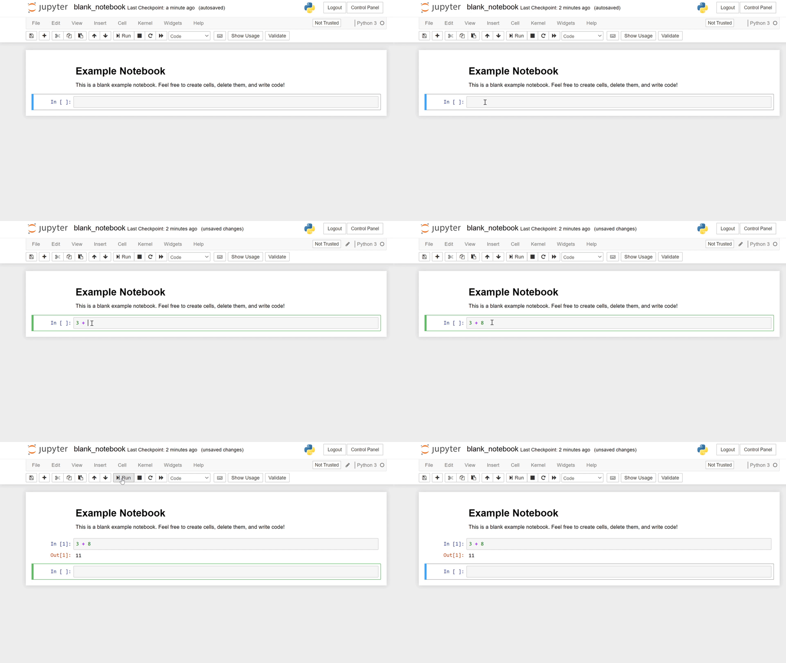
to perform a basic computation. Click inside the cell to select it, and type 3 + 8, as shown below:

Fig. 2.1 Running a code cell in a notebook.
Congratulations! You’ve written your first piece of python code. You can run your code in one of two ways:
By clicking the “Run” button in the toolbar. This will run the cell that is currently selected (and only that cell).
Note
If you do not see the toolbar, select “View -> Toggle Toolbar” in the menu at the top of the notebook.
By pressing Shift + Return. This is our preferred way, since it is faster than reaching for the mouse.
Upon running the cell, you’ll see the answer appear directly below. Additionally, a new empty code cell has been created for us. Go ahead and write some arithmetic in the new cell and run it.
Code cells can be changed after they are executed. Suppose that we made a
mistake when writing out first code cell, and that we really meant to compute
30 + 8 instead of 3 + 8. Select the first code cell, change the text to read
30 + 8, and run it again. You’ll notice that the output is replaced by the new
correct result.
Jupyter Tip
Any changes you make to the notebook will be automatically saved at regular intervals, but you can save them immediately by selecting “File -> Save and Checkpoint”.
2.2. Markdown Cells
Jupyter notebooks can also include rich text cells. These are useful for writing explanations to go along with your code. The text in these cells can be formatted by using Markdown.
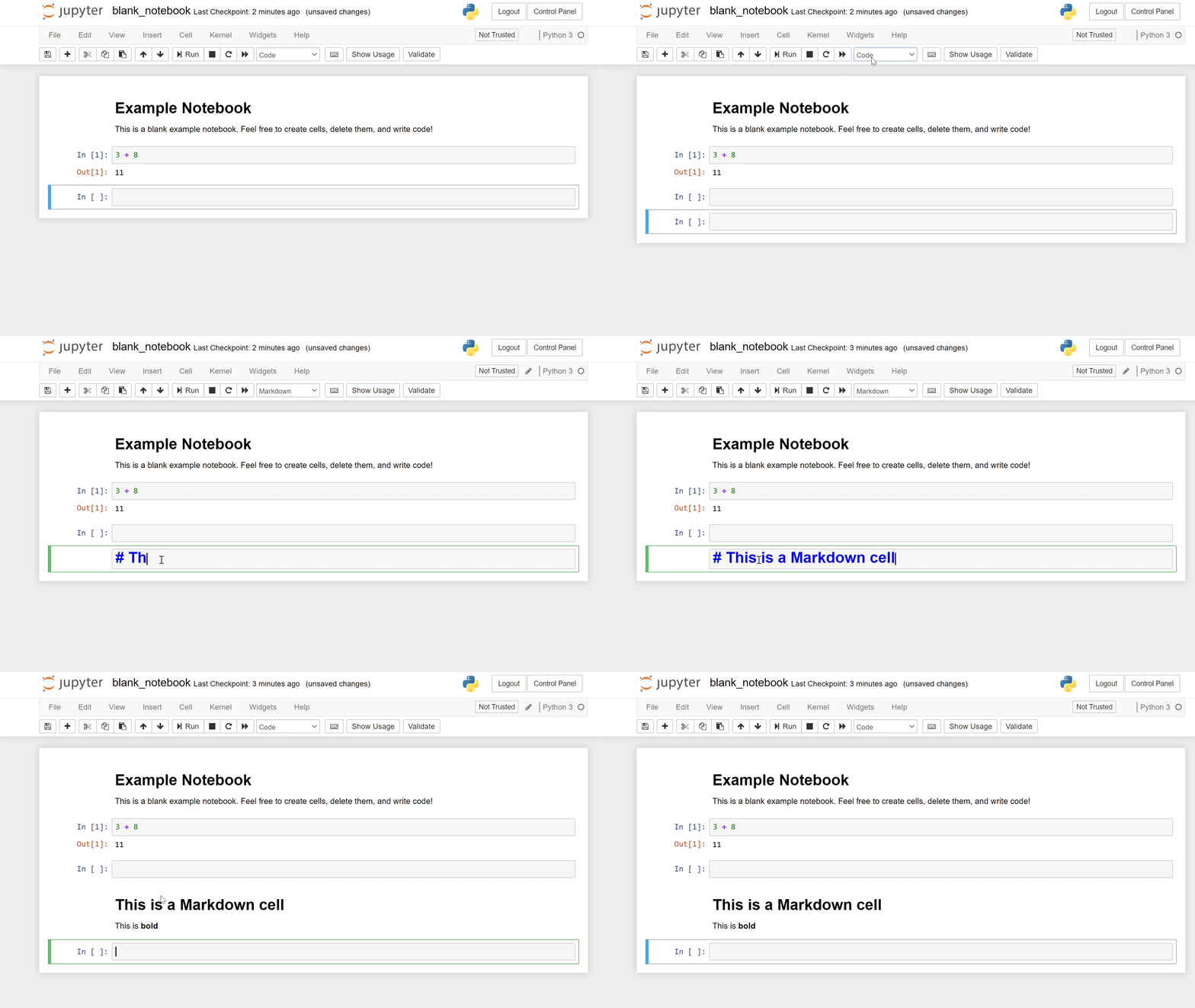
Create a new cell by clicking the “+” button in the toolbar, or by selecting “Insert -> Insert Cell Below” from the menu. Then, with the new cell selected, select “Markdown” from the dropdown box shown in the toolbar.
Jupyter Tip
There are plenty of keyboard shortcuts to use with Jupyter notebooks. One of the most useful is Ctrl-m a, which creates a new cell. Another useful shortcut is dd, which deletes the selected cell. Select “Help -> Keyboard shortcuts” to see all of them.
Now copy and paste the below directly into the new cell:
# This is a header

I can make words **bold** with two asterisks!

This is a [link](www.google.com).

And this is some advanced math:

$$
e^{\pi i} = -1
$$
“Run” the cell. You’ll notice that the text is now nicely formatted, complete with a header, bold text, a link, and even some nicely-displayed mathematical notation.

Fig. 2.2 Running a markdown cell in a notebook.
You can double-click the cell to see and edit its Markdown source once again.
You will not be asked to use Markdown in the rest of the course, but text cells are very useful part of Jupyter notebooks.