11. GroupBy¶

What is the most common cause of wildfires in California? We can count the number of fires due to a particular cause, such as lightning, using a query:

calfire[calfire.get('cause') == '1 - Lightning'].shape[0]

This query retrieves a table containing only those fires caused by lightning, and .shape[0] returns the number of rows in this table, effectively counting the number of such fires. To determine the number of fires due to each cause, we could write a query for each different type of fire:

calfire[calfire.get('cause') == '1 - Lightning'].shape[0]
calfire[calfire.get('cause') == '2 - Equipment Use'].shape[0]
calfire[calfire.get('cause') == '3 - Smoking'].shape[0]
...
calfire[calfire.get('cause') == '14 - Unknown'].shape[0]

But there is a better way. As we’ll see in this section, the powerful .groupby method allows to quickly group a table’s rows and perform the same analysis on each group.

11.1. Split, Aggregate, Combine¶

Let’s count the number of fires due to each cause using .groupby:

calfire.groupby('cause').count()

	year	month	name	acres	county	longitude	latitude
cause
1 - Lightning	2550	2550	2550	2550	2550	2550	2550
10 - Vehicle	399	399	399	399	399	399	399
11 - Powerline	359	359	359	359	359	359	359
12 - Firefighter Training	2	2	2	2	2	2	2
13 - Non-Firefighter Training	5	5	5	5	5	5	5
...	...	...	...	...	...	...	...
5 - Debris	610	610	610	610	610	610	610
6 - Railroad	70	70	70	70	70	70	70
7 - Arson	763	763	763	763	763	763	763
8 - Playing with fire	151	151	151	151	151	151	151
9 - Miscellaneous	1603	1603	1603	1603	1603	1603	1603

17 rows × 7 columns

This result tells us that there were 2550 fires caused by lightning, 399 caused by vehicles, and so forth. But why do all of the columns contain exactly the same information? And what is going on with the column labels? Let’s dissect this piece of code to understand what, exactly, is going on.

Three things happen when we run calfire.groupby('cause').count():

The table’s rows are split into groups according to cause. All of the rows whose cause is '1 - Lightning' are placed into one group, all of the rows whose cause is '2 - Equipment Use' are placed into another group and so on.
Each group is aggregated into a single row by counting the number of entries in each of the group’s columns.
The resulting rows are combined to form a new table, with one row for every group.

Fig. 11.1 below demonstrates this process on a small example table.

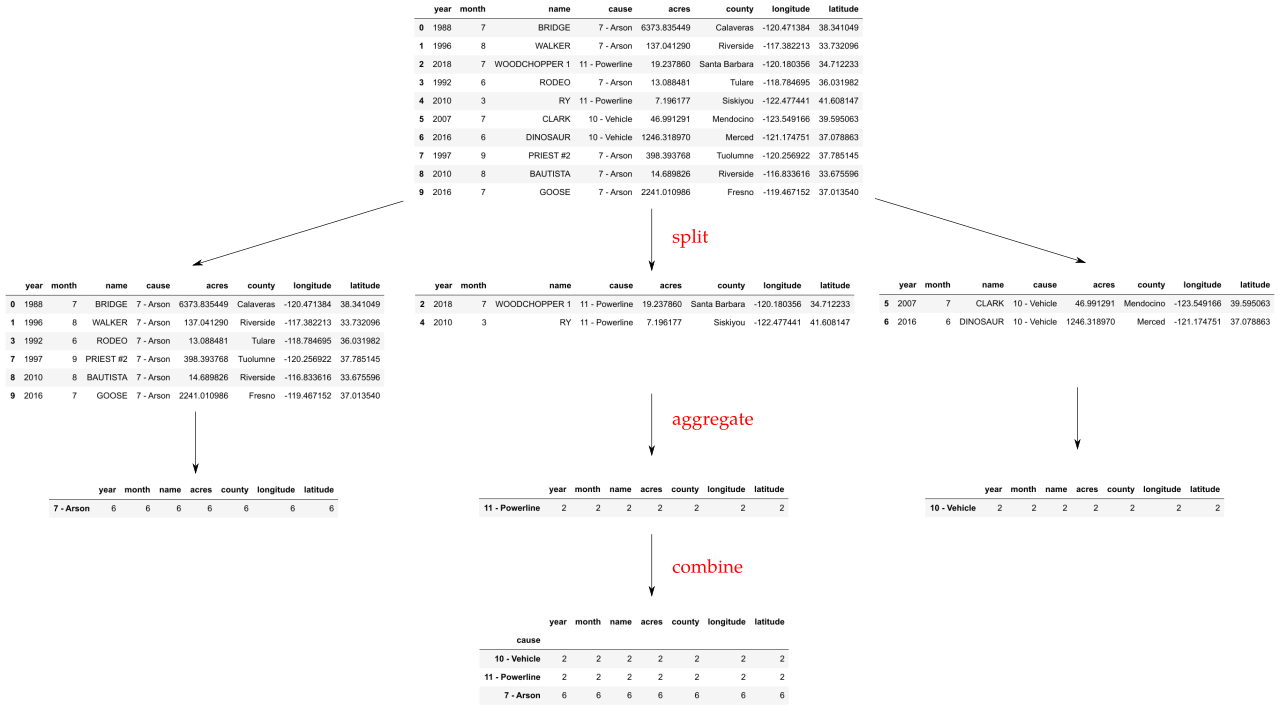
Fig. 11.1 caption: The split-aggregate-combine pattern.¶

11.1.1. `.groupby`¶

The “split” part of the “split-aggregate-combine” process is performed by the .groupby method. It accepts a single argument: the column whose values should be used to form groups. When we call .groupby('cause'), babypandas looks through our table and separates the rows into groups by their value in the cause column – all of the rows whose cause is '1 - Lightning' are placed into one group, all of the rows whose cause is '2 - Equipment Use' are placed into another group and so on.

The result of .groupby is something called a DataFrameGroupby object:

calfire.groupby('cause')

<babypandas.bpd.DataFrameGroupBy at 0x7f9b600a4460>

A DataFrameGroupBy object doesn’t look all that useful by itself. We need to tell babypandas what action should be taken on each group. We do this by specifying an aggregator.

11.1.2. Aggregators¶

After we have grouped the table’s rows using .groupby, we must next apply an aggregator. An aggregator takes each group, aggregates it into a single row, and finally combines these rows to form a new table, with one row for each group with the group’s name as its label. There are several aggregators to choose from, namely:

.mean()
.median()
.max()
.min()
.count()

We have already seen how the .count() aggregator can be used to count the number of fires due to each cause. If we instead wanted to find the average size of each type of fire, we could use the .mean() aggregator:

calfire.groupby('cause').mean()

	year	month	acres	longitude	latitude
cause
1 - Lightning	1993.815294	7.480784	2436.783344	-120.810116	39.036871
10 - Vehicle	2008.689223	7.343358	1456.904712	-120.205692	36.708733
11 - Powerline	2006.729805	7.200557	1441.556715	-120.465738	36.601976
12 - Firefighter Training	2002.500000	8.000000	1082.385803	-120.401002	38.392531
13 - Non-Firefighter Training	2001.800000	3.800000	305.873876	-119.927214	34.978246
...	...	...	...	...	...
5 - Debris	1977.645902	7.457377	992.116907	-121.751834	39.450188
6 - Railroad	1997.042857	7.300000	1267.831665	-120.741341	38.573846
7 - Arson	1995.422018	7.546527	2509.532333	-120.137300	37.265328
8 - Playing with fire	1995.052980	7.039735	753.464156	-119.490352	36.122455
9 - Miscellaneous	1988.960075	7.471616	2901.573769	-119.527044	36.746385

17 rows × 5 columns

The average size of each kind of fire is contained in the 'acres' column.

When an aggregator is applied to a group, it performs its operation on each column independently. For example, the .mean() aggregator computes the mean of the 'year' column, the mean of the 'month' column, and so forth. So what we see in the table above is the mean year of all fires caused by lightning, the mean month, mean size in acres, and so on.

Notice that some columns are apparently missing. For instance, the original table has columns called 'name' and 'county', but the table above does not have these columns. This is because they contain strings, and it doesn’t make sense to find the mean of a collection of strings. As such, babypandas has automatically dropped these column from the result. Likewise, these columns will be dropped if we use the .sum() aggregator.

What if we use the .max() aggregator? You might be surprised to find the 'name' and 'county' columns in the result:

calfire.groupby('cause').max()

	year	month	name	acres	county	longitude	latitude
cause
1 - Lightning	2019	12	ZIEGLER-Iron Complex	315511.500000	Yuba	-114.987792	41.990849
10 - Vehicle	2019	12	ZACA	229651.406250	Yuba	-115.569205	41.874351
11 - Powerline	2019	12	YUBA	153335.562500	Yuba	-116.395032	41.925561
12 - Firefighter Training	2004	8	OREGON	1954.705933	Fresno	-119.301603	39.597129
13 - Non-Firefighter Training	2003	6	UNIT #5	805.634644	Monterey	-118.426778	35.824536
...	...	...	...	...	...	...	...
5 - Debris	2019	12	ZIEBRIGHT	161815.656250	Yuba	-115.393351	41.995821
6 - Railroad	2016	11	WOODHOUSE	56076.332031	Yuba	-116.193409	41.979014
7 - Arson	2019	12	YOLO	160833.109375	Yuba	-116.072059	41.992000
8 - Playing with fire	2019	11	YORBA LINDA	38347.472656	Yuba	-116.308956	41.997899
9 - Miscellaneous	2019	12	ZERMATT	281790.875000	Yuba	-114.478988	42.002868

17 rows × 7 columns

Here, babypandas adopts the view that the maximum of a collection of strings is the last string in the alphabetical ordering. So for instance, the ZACA fire was the fire whose name was alphabetically last among all fires caused by vehicles. Likewise, the .min() aggregator will produce the name that is alphabetically first within the group.

Warning

The aggregator is applied to each column independently. A common mistake is to believe that, after running calfire.groupby('cause').max(), the 'acres' column will contain the size of the largest fire in each group, and the 'name' column contains its name. This is not the case: the 'name' column contains the name that appears last in the alphabetical ordering of names within the group.

Let’s take another look at the count aggregator. Recall the result of our first groupby:

calfire.groupby('cause').count()

	year	month	name	acres	county	longitude	latitude
cause
1 - Lightning	2550	2550	2550	2550	2550	2550	2550
10 - Vehicle	399	399	399	399	399	399	399
11 - Powerline	359	359	359	359	359	359	359
12 - Firefighter Training	2	2	2	2	2	2	2
13 - Non-Firefighter Training	5	5	5	5	5	5	5
...	...	...	...	...	...	...	...
5 - Debris	610	610	610	610	610	610	610
6 - Railroad	70	70	70	70	70	70	70
7 - Arson	763	763	763	763	763	763	763
8 - Playing with fire	151	151	151	151	151	151	151
9 - Miscellaneous	1603	1603	1603	1603	1603	1603	1603

17 rows × 7 columns

Notice that all of the columns contain exactly the same information. We now know why this is: when we apply .count(), it counts the number of entries within the 'year' column, the 'month' column, 'name' column, etc. There are the name number of entries within each column, so we get the same number for each. Also notice that the column names are no longer very meaningful. The 'year' column no longer contains years – it contains the count of entries in the 'year' column within each group.

If our goal is to count the number of fires due to each cause, we could use any column in the result – I usually just pick the one that is easiest to type:

calfire.groupby('cause').count().get('year')

cause
- Lightning                    2550
- Vehicle                      399
- Powerline                    359
- Firefighter Training           2
- Non-Firefighter Training       5
                                 ... 
- Debris                        610
- Railroad                       70
- Arson                         763
- Playing with fire             151
- Miscellaneous                1603
Name: year, Length: 17, dtype: int64

11.2. Examples¶

Which year had the largest number of fires?

We can count the number of fires from each year with .groupby() and .count(). But this time we want to group by the year column, so that fires from the same year are placed within the same group.

calfire.groupby('year').count()

	month	name	cause	acres	county	longitude	latitude
year
1898	3	3	3	3	3	3	3
1902	1	1	1	1	1	1	1
1903	1	1	1	1	1	1	1
1908	2	2	2	2	2	2	2
1909	2	2	2	2	2	2	2
...	...	...	...	...	...	...	...
2015	286	286	286	286	286	286	286
2016	342	342	342	342	342	342	342
2017	591	591	591	591	591	591	591
2018	397	397	397	397	397	397	397
2019	295	295	295	295	295	295	295

115 rows × 7 columns

Notice that the index now contains the different years, since we have grouped by year. To find the year with the largest number of fires, we’ll do what we’ve done before: sort the table and return the last entry in the index:

calfire.groupby('year').count().sort_values(by='month').index[-1]

If you’re confused why we are sorting by the 'month' column, remember: all of the columns contain the exact same information after .count()! So we could have sorted by the 'county' column to get the same result:

calfire.groupby('year').count().sort_values(by='county').index[-1]

What is the median fire size in each county?

We’ll group by the 'county' column, and apply the .median() aggregator:

calfire.groupby('county').median()

	year	month	acres	longitude	latitude
county
Alameda	1988.0	7.0	346.514191	-121.624947	37.707623
Alpine	2012.0	8.0	186.335419	-119.822902	38.443338
Amador	1992.5	7.0	240.124207	-120.666797	38.438166
Butte	1999.0	8.0	471.250946	-121.559119	39.634084
Calaveras	1991.0	8.0	228.224197	-120.597127	38.180825
...	...	...	...	...	...
Tulare	1996.0	7.0	167.007103	-118.773436	36.336689
Tuolumne	2001.0	8.0	86.326668	-120.047074	37.946170
Ventura	1996.0	8.0	122.332626	-119.021737	34.333966
Yolo	1988.0	7.0	677.440491	-122.097986	38.744614
Yuba	2008.0	7.5	74.831673	-121.341850	39.201832

57 rows × 5 columns

If we want just the fire size, we could .get the 'acres' column:

calfire.groupby('county').median().get('acres')

county
Alameda      346.514191
Alpine       186.335419
Amador       240.124207
Butte        471.250946
Calaveras    228.224197
                ...    
Tulare       167.007103
Tuolumne      86.326668
Ventura      122.332626
Yolo         677.440491
Yuba          74.831673
Name: acres, Length: 57, dtype: float64

What was the size of the largest fire in 1995?

We will group by year and apply the max aggregator:

calfire.groupby('year').max()

	month	name	cause	acres	county	longitude	latitude
year
1898	9	MATILIJA	14 - Unknown	20539.949219	Ventura	-119.265380	34.488614
1902	8	FEROUD	14 - Unknown	731.481567	Ventura	-119.320979	34.417515
1903	10	SAN ANTONIO	14 - Unknown	380.260590	Ventura	-119.253422	34.430616
1908	9	REEVES	14 - Unknown	7433.901855	Ventura	-119.179959	41.000197
1909	9	SHOEMAKER	14 - Unknown	3174.514648	Ventura	-117.685816	34.482616
...	...	...	...	...	...	...	...
2015	12	ZEBRA	9 - Miscellaneous	151546.812500	Yuba	-115.837487	41.989971
2016	12	YUCCA	9 - Miscellaneous	132104.281250	Yuba	-116.557240	41.971890
2017	12	ZERMATT	9 - Miscellaneous	281790.875000	Yuba	-115.268126	42.002868
2018	12	YOSEMITE	9 - Miscellaneous	410202.468750	Yuba	-116.359866	41.979459
2019	12	WILLOWS 3	9 - Miscellaneous	77762.140625	Yuba	-115.339065	42.007182

115 rows × 7 columns

Now we want to retrieve the size (in acres) of the fire from 1995. We’ll do this with our familiar .get().loc[] pattern:

calfire.groupby('year').max().get('acres').loc[1995]

21444.125

Tip

When method chaining, it is useful to keep in mind what type of object you are working with at each step. Any time you write ., you should be able to stop and say whether the piece of code to the left evaluates to a table, a series, a number, etc. For instance, calfire.groupby('year').max() evaluates to a table, so whatever follows should be a table method.

11.3. `.groupby` versus querying¶

In the last example above, we found the size of the largest fire from 1995. We did this with .groupby() and the .max() aggregator. While this worked, you might have noticed that we can obtain the same result with a simple query:

calfire[calfire.get('year') == 1995].sort_values(by='acres').get('acres').iloc[-1]

21444.125

Which is better? And how do we choose which method to use?

In many cases like this one, both approaches work equally well. In general, however, queries are most useful when asking a question about a single group (or subset) of a table, and .groupby is most useful when your question is about each group. As a rule of thumb, if you question contains the word “each” – like in “What was the size of the largest fire in each county?” – you probably want to use .groupby.

Queries have many advantages over .groupby. For one, queries can be performed with complex, compound conditions, while .groupby’s is limited to forming groups using the values in a particular column. For instance, suppose we want to find the size of the largest fire between 1990 and 2000. We can do this with a query, but not with .groupby directly. Second, a query results in a full DataFrame object, while .groupby must be followed by one of a limited number of available aggregators.

Jupyter Tip

If you’d like to know how efficient a particular piece of code is, you can use the %%timeit “magic function”. This runs a cell over and over, printing the average time it takes to execute. Create a new cell with %%timeit and the code you’d like to time, like so:

%%timeit
calfire.groupby('year').max().get('acres').loc[1995]

This will print something like the following:

62.4 ms ± 161 µs per loop (mean ± std. dev. of 7 runs, 10 loops each)

This tells us that the code took 62.4 milliseconds to run on average. Not bad!

11.4. Subgroups¶

Which month of which year had the most wildfires in California history? To answer this question, we’d like to count the number of wildfires for each month of every year. So for instance, the number of fires in January 1991, February 1991, …, January 1992, February 1992, …, and so on.

This looks like a job for .groupby with the .count aggregator. But what do we group by? If we group by year, we’ll get the number of fires in each year. If we just group by month, we’ll get the number of fires in each month over all years, which isn’t quite what we want:

calfire.groupby('month').count()

	year	name	cause	acres	county	longitude	latitude
month
1	119	119	119	119	119	119	119
2	85	85	85	85	85	85	85
3	131	131	131	131	131	131	131
4	274	274	274	274	274	274	274
5	832	832	832	832	832	832	832
...	...	...	...	...	...	...	...
8	2945	2945	2945	2945	2945	2945	2945
9	2179	2179	2179	2179	2179	2179	2179
10	966	966	966	966	966	966	966
11	424	424	424	424	424	424	424
12	169	169	169	169	169	169	169

12 rows × 7 columns

What we’d like to do is to group rows which are in the same year and in the same month. It turns out that .groupby supports this via subgrouping. We can specify two columns to group by using a list. First, “outer” groups will be formed using the first column, then “inner” groups will be formed within each outer group using the values in the second column. Here is how it looks in action:

calfire.groupby(['year', 'month']).count()

		name	cause	acres	county	longitude	latitude
year	month
1898	4	1	1	1	1	1	1
1898	9	2	2	2	2	2	2
1902	8	1	1	1	1	1	1
1903	10	1	1	1	1	1	1
1908	7	1	1	1	1	1	1
...	...	...	...	...	...	...	...
2019	8	41	41	41	41	41	41
	9	68	68	68	68	68	68
	10	41	41	41	41	41	41
	11	15	15	15	15	15	15
	12	1	1	1	1	1	1

931 rows × 6 columns

We see something new in the result: both the year and the month are being used as the row label. This called a hierarchical index (or multi-index). Hierarchical indices are quite powerful, but introduce extra complexity. Instead of using multi-indexes, we’ll use the .reset_index() method to move each level of the index to its own column:

by_month = calfire.groupby(['year', 'month']).count().reset_index()
by_month

	year	month	name	cause	acres	county	longitude	latitude
0	1898	4	1	1	1	1	1	1
1	1898	9	2	2	2	2	2	2
2	1902	8	1	1	1	1	1	1
3	1903	10	1	1	1	1	1	1
4	1908	7	1	1	1	1	1	1
...	...	...	...	...	...	...	...	...
926	2019	8	41	41	41	41	41	41
927	2019	9	68	68	68	68	68	68
928	2019	10	41	41	41	41	41	41
929	2019	11	15	15	15	15	15	15
930	2019	12	1	1	1	1	1	1

931 rows × 8 columns

Which month of which year had the most wildfires? We’ll solve this by sorting, as usual:

by_month_sorted = by_month.sort_values(by='name')

by_month_sorted.get('year').iloc[-1]

by_month_sorted.get('month').iloc[-1]

Notes on (Baby)Pandas

GroupBy

Contents

11. GroupBy¶

11.1. Split, Aggregate, Combine¶

11.1.1. `.groupby`¶

11.1.2. Aggregators¶

11.2. Examples¶

11.3. `.groupby` versus querying¶

11.4. Subgroups¶

Notes on (Baby)Pandas

GroupBy

Contents

11. GroupBy¶

11.1. Split, Aggregate, Combine¶

11.1.1. .groupby¶

11.1.2. Aggregators¶

11.2. Examples¶

11.3. .groupby versus querying¶

11.4. Subgroups¶

11.1.1. `.groupby`¶

11.3. `.groupby` versus querying¶